r5py: Case Brighton - Calculate travel time matrices in Python
Contents
r5py: Case Brighton - Calculate travel time matrices in Python#
Lesson objectives#
This tutorial focuses on introducing you how to compute travel time matrices by different travel modes using a new Python library called r5py (still a work in progress). Travel time data is fundamental information whenever aiming to analyze e.g. accessibility -related questions.
Library status#
r5py is still very much a work in progress but it already has core functionalities available to compute travel time matrices that are relevant to spatial accessibility analysis. r5py is still missing many of the functionalities of r5r, but eventually, both of these libraries aim to provide a similar set of functionalities.
Run these codes in Binder#
Before you can run this Notebook, and/or do any programming, you need to launch the Binder instance. You can find buttons for activating the python environment at the top-right of this page which look like this:

Working with Jupyter Notebooks#
Jupyter Notebooks are documents that can be used and run inside the JupyterLab programming environment containing the computer code and rich text elements (such as text, figures, tables and links).
A couple of hints:
You can execute a cell by clicking a given cell that you want to run and pressing Shift + Enter (or by clicking the “Play” button on top)
You can change the cell-type between
Markdown(for writing text) andCode(for writing/executing code) from the dropdown menu above.
See further details and help for using Notebooks and JupyterLab from here.
Compute travel time matrices#
When trying to understand the accessibility of a specific location, you typically want to look at travel times between multiple locations (one-to-many). Next, we will learn how to calculate travel time matrices using r5py Python library.
When calculating travel times with r5py, you typically need a couple of datasets:
A road network dataset from OpenStreetMap (OSM) in Protocolbuffer Binary (
.pbf) format:This data is used for finding the fastest routes and calculating the travel times based on walking, cycling and driving. In addition, this data is used for walking/cycling legs between stops when routing with transit.
Hint: Sometimes you might need modify the OSM data beforehand, e.g., by cropping the data or adding special costs for travelling (e.g., for considering slope when cycling/walking). When doing this, you should follow the instructions on the Conveyal website. For adding customized costs for pedestrian and cycling analyses, see this repository.
A transit schedule dataset in General Transit Feed Specification (GTFS.zip) format (optional):
This data contains all the necessary information for calculating travel times based on public transport, such as stops, routes, trips and the schedules when the vehicles are passing a specific stop. You can read about the GTFS standard here.
Hint:
r5pycan also combine multiple GTFS files, as sometimes you might have different GTFS feeds representing, e.g., the bus and metro connections.
Sample datasets#
In the following tutorial, we use open source datasets for Brighton & Hove:
The point dataset for this tutorial has been obtained from WorldPop -project licensed under a Creative Commons Attribution 4.0 International License.
The street network is a cropped and filtered extract of OpenStreetMap (© OpenStreetMap contributors, ODbL license)
The GTFS transport schedule dataset for Brighton are open datasets obtained from:
Bus schedules: Brighton & Hove Bus and Coach Company licensed under Open Government License Version 3.0.
Download the datasets#
We have prepared a Zip-package with all relevant data that helps you to start working with the tools quickly. You can download and extract the data by executing the following commands:
# Download the data from a S3 bucket into 'data' folder
!wget -P data/ https://a3s.fi/swift/v1/AUTH_0914d8aff9684df589041a759b549fc2/R5edu/Brighton.zip

# Extract the contents
!unzip -q data/Brighton.zip -d data/
--2022-11-29 21:45:08--  https://a3s.fi/swift/v1/AUTH_0914d8aff9684df589041a759b549fc2/R5edu/Brighton.zip
Resolving a3s.fi (a3s.fi)... 86.50.254.19, 86.50.254.18
Connecting to a3s.fi (a3s.fi)|86.50.254.19|:443... connected.
HTTP request sent, awaiting response... 200 OK
Length: 68301274 (65M) [application/zip]
Saving to: ‘data/Brighton.zip’

Brighton.zip        100%[===================>]  65,14M  36,2MB/s    in 1,8s

2022-11-29 21:45:10 (36,2 MB/s) - ‘data/Brighton.zip’ saved [68301274/68301274]
If running the cell above does not work for some reason (on your local computer), you can manually download the data. If you do this, extract the contents of the Zip file (Brighton.zip) into the <YOUR_FOLDER_CONTAINING_THIS_NOTEBOOK>/data -folder.
Load the origin and destination data#
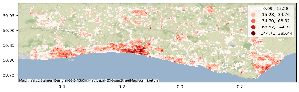
Let’s start by downloading a sample point dataset into a geopandas GeoDataFrame that we can use as our origin and destination locations. For the sake of this exercise, we have prepared a grid of points covering parts of Sussex. The point data also contains the number of residents of each 100 meter cell:
import geopandas as gpd
import contextily as cx

# Load population points
pop_fp = "data/Brighton/Brighton_pop_points_2020.gpkg"
pop_points = gpd.read_file(pop_fp)

ax = pop_points.plot("population", scheme="natural_breaks", cmap="Reds", figsize=(12,12), legend=True, markersize=3.5)
cx.add_basemap(ax, crs=pop_points.crs)
Let’s also check how the attribute table of the data looks like:
# Check the first 5 rows
pop_points.head()
| x | y | population | id | geometry | |
|---|---|---|---|---|---|
| 0 | -0.499167 | 50.972500 | 10.112679 | 0 | POINT (-0.49917 50.97250) |
| 1 | -0.499167 | 50.971667 | 19.579712 | 1 | POINT (-0.49917 50.97167) |
| 2 | -0.499167 | 50.970833 | 12.178864 | 2 | POINT (-0.49917 50.97083) |
| 3 | -0.499167 | 50.968333 | 5.552000 | 3 | POINT (-0.49917 50.96833) |
| 4 | -0.499167 | 50.967500 | 2.551825 | 4 | POINT (-0.49917 50.96750) |
Next, we will geocode the address for Brighton Railway station. For doing this, we can use oxmnx library and its handy .geocode() -function:
import osmnx as ox
from shapely.geometry import Point

# Find coordinates of the main railway station
lat, lon = ox.geocode("Railway station, Brighton")

# Create a GeoDataFrame out of the coordinates
station = gpd.GeoDataFrame({"geometry": [Point(lon, lat)], "name": "Brighton Railway station", "id": [0]}, index=[0], crs="epsg:4326")
station.explore(max_zoom=14, color="red", marker_kwds={"radius": 12})
Next, we will prepare the routable network
%%time
# Allow 6 GB memory
import sys
sys.argv.append(["--max-memory", "6G"])

import datetime
from r5py import TransportNetwork, TravelTimeMatrixComputer, TransitMode, LegMode

# Filepath to OSM data
osm_fp = "data/Brighton/brightonhove.pbf"

transport_network = TransportNetwork(
    osm_fp,
    [
        "data/Brighton/brightonhove_1667288932.zip"
    ]
)
WARNING: An illegal reflective access operation has occurred
WARNING: Illegal reflective access by org.mapdb.Volume$ByteBufferVol (file:/home/hentenka/.cache/r5py/r5-v6.6-all.jar) to method java.nio.DirectByteBuffer.cleaner()
WARNING: Please consider reporting this to the maintainers of org.mapdb.Volume$ByteBufferVol
WARNING: Use --illegal-access=warn to enable warnings of further illegal reflective access operations
WARNING: All illegal access operations will be denied in a future release
CPU times: user 1min 24s, sys: 2.15 s, total: 1min 26s
Wall time: 29.4 s
After this step, we can do the routing
travel_time_matrix_computer = TravelTimeMatrixComputer(
    transport_network,
    origins=station,
    destinations=pop_points,
    departure=datetime.datetime(2022,12,1,7,30),
    transport_modes=[TransitMode.TRANSIT, LegMode.WALK],
)
travel_time_matrix = travel_time_matrix_computer.compute_travel_times()
Warning: SIGINT handler expected:libjvm.so+0xc2ddc0  found:0x0000000000000001
Running in non-interactive shell, SIGINT handler is replaced by shell
Signal Handlers:
SIGSEGV: [libjvm.so+0xc2d970], sa_mask[0]=11111111011111111101111111111110, sa_flags=SA_RESTART|SA_SIGINFO
SIGBUS: [libjvm.so+0xc2d970], sa_mask[0]=11111111011111111101111111111110, sa_flags=SA_RESTART|SA_SIGINFO
SIGFPE: [libjvm.so+0xc2d970], sa_mask[0]=11111111011111111101111111111110, sa_flags=SA_RESTART|SA_SIGINFO
SIGPIPE: [libjvm.so+0xc2d970], sa_mask[0]=11111111011111111101111111111110, sa_flags=SA_RESTART|SA_SIGINFO
SIGXFSZ: [libjvm.so+0xc2d970], sa_mask[0]=11111111011111111101111111111110, sa_flags=SA_RESTART|SA_SIGINFO
SIGILL: [libjvm.so+0xc2d970], sa_mask[0]=11111111011111111101111111111110, sa_flags=SA_RESTART|SA_SIGINFO
SIGUSR2: [libjvm.so+0xc2dc60], sa_mask[0]=00000000000000000000000000000000, sa_flags=SA_RESTART|SA_SIGINFO
SIGHUP: [libjvm.so+0xc2ddc0], sa_mask[0]=11111111011111111101111111111110, sa_flags=SA_RESTART|SA_SIGINFO
SIGINT: SIG_IGN, sa_mask[0]=00000000000000000000000000000000, sa_flags=SA_ONSTACK
SIGTERM: [libjvm.so+0xc2ddc0], sa_mask[0]=11111111011111111101111111111110, sa_flags=SA_RESTART|SA_SIGINFO
SIGQUIT: [libjvm.so+0xc2ddc0], sa_mask[0]=11111111011111111101111111111110, sa_flags=SA_RESTART|SA_SIGINFO
Now we can join the travel time information back to the population grid
geo = pop_points.merge(travel_time_matrix, left_on="id", right_on="to_id")
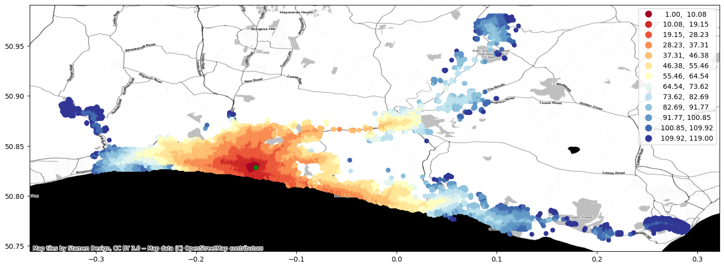
Finally, we can visualize the travel time map and investigate how the railway station in Brighton can be accessed from different parts of the region, by public transport.
import contextily as cx
ax = geo.plot(column="travel_time", cmap="RdYlBu", scheme="equal_interval", k=13, legend=True, figsize=(18,18))
ax = station.to_crs(crs=geo.crs).plot(ax=ax, color="green", markersize=40)
cx.add_basemap(ax, crs=geo.crs, source=cx.providers.Stamen.Toner)
Calculate travel times by bike#
In a very similar manner, we can calculate travel times by cycling. We only need to modify our TravelTimeMatrixComputer object a little bit. We specify the cycling speed by using the parameter speed_cycling and we change the transport_modes parameter to correspond to [LegMode.BICYCLE. This will initialize the object for cycling analyses:
tc_bike = TravelTimeMatrixComputer(
    transport_network,
    origins=station,
    destinations=pop_points,
    speed_cycling=16,
    transport_modes=[LegMode.BICYCLE],
)
ttm_bike = tc_bike.compute_travel_times()
Let’s again make a table join with the population grid
geo = pop_points.merge(ttm_bike, left_on="id", right_on="to_id")
And plot the data
ax = geo.plot(column="travel_time", cmap="RdYlBu", scheme="equal_interval", k=13, legend=True, figsize=(18,18))
ax = station.to_crs(crs=geo.crs).plot(ax=ax, color="green", markersize=40)
cx.add_basemap(ax, crs=geo.crs, source=cx.providers.Stamen.Toner)

Calculate catchment areas#
One quite typical accessibility analysis is to find out catchment areas for multiple locations, such as schools. In the below, we will extract all schools in Brighton area and calculate travel times from all grid cells to the closest one. As a result, we have catchment areas for each school.
Let’s start by preparing data. In the following, we will:
Download OSM data about locations of schools in Brighton area, using
osmnx.Some of the downloaded geometries might be in Polygon format, so we need to convert them into points by calculating their centroid
We will also add a column
idfor the data which is required byr5py(as well asr5r)
import osmnx as ox
from shapely.geometry import box

# Extent of the data for Brighton
# (minx, miny, maxx, maxy)
bounds = (-0.49975, 50.73,  0.3469234, 50.98)

# Create a GeoDataFrame
gdf = gpd.GeoDataFrame(geometry=[box(*bounds)], crs="EPSG:4326")
gdf.explore()

# Download schools from OpenStreetMap
tags = {"amenity": "school"}
schools = ox.geometries_from_polygon(gdf.geometry.values[0], tags)

# Use centroid as geometry (we ignore the shape of the building)
schools["geometry"] = schools.centroid

# Add a unique id column based on the index
schools["id"] = schools.index.droplevel(level=0)

# Plot to map
schools.explore()
/tmp/ipykernel_535156/1593569817.py:17: UserWarning: Geometry is in a geographic CRS. Results from 'centroid' are likely incorrect. Use 'GeoSeries.to_crs()' to re-project geometries to a projected CRS before this operation.

  schools["geometry"] = schools.centroid
Next, we can initialize our travel time matrix calculator using the schools as the origins:
travel_time_matrix_computer = TravelTimeMatrixComputer(
    transport_network,
    origins=schools,
    destinations=pop_points,
    departure=datetime.datetime(2022,12,1,8,30),
    transport_modes=[TransitMode.TRANSIT, LegMode.WALK],
)
travel_time_matrix = travel_time_matrix_computer.compute_travel_times()
travel_time_matrix.shape
(13250240, 3)
As we can see, there are approx. 1.3 million rows of data, which comes as a result of the connections between origins and destinations. Next, we want aggregate the data and keep only travel time information to the closest school:
# Find out the travel time to closest school
closest = travel_time_matrix.groupby("to_id")["travel_time"].min().reset_index()
closest.head()
| to_id | travel_time | |
|---|---|---|
| 0 | 0 | 42.0 |
| 1 | 1 | 39.0 |
| 2 | 2 | 40.0 |
| 3 | 3 | 41.0 |
| 4 | 4 | 42.0 |
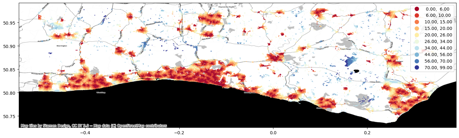
Then we can make a table join with the grid in a similar manner as previously and visualize the data:
geo = pop_points.merge(closest, left_on="id", right_on="to_id")
import contextily as cx
ax = geo.plot(column="travel_time", cmap="RdYlBu", scheme="natural_breaks", k=10, legend=True, figsize=(18,18), markersize=0.2)
cx.add_basemap(ax, crs=geo.crs, source=cx.providers.Stamen.Toner)
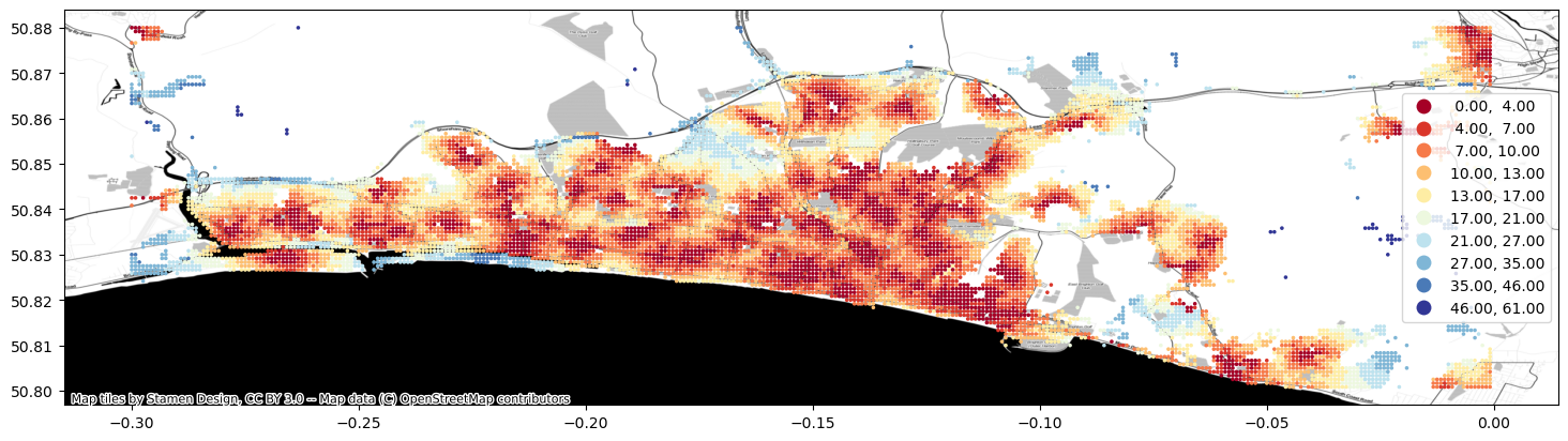
# Make a zoom-in map - .cx is used to limit the data based on minx: maxx, miny: maxy
ax = geo.cx[-0.3: 0, 50.8: 50.88].plot(column="travel_time", cmap="RdYlBu", scheme="natural_breaks", k=10, legend=True, figsize=(18,18), markersize=2.5)
cx.add_basemap(ax, crs=geo.crs, source=cx.providers.Stamen.Toner)
# Make an interactive map - .cx is used to limit the data based on minx: maxx, miny: maxy
# Note: Be careful not to plot a large area of points, because the interactive plotting uses a lot of memory
geo.cx[-0.2: -0.1, 50.8: 50.88].explore(column="travel_time", cmap="RdYlBu",
                                        scheme="natural_breaks", k=10, legend=True,
                                        marker_kwds={"radius": 2.5})
That’s it! As you can, see now we have a nice map showing the catchment areas for each school.