r5r: Accounting for monetary costs#

This tutorial shows how to configure and use custom fare rules in order to account for monetary travel costs when generating travel time matrices and accessibility estimates with the r5r package.

Credits:

This tutorial is a direct copy from r5r -documentation made by r5r contributors.

Getting started#

Run these codes in Binder#

Before you can run this Notebook, and/or do any programming, you need to launch the Binder instance. You can find buttons for activating the python environment at the top-right of this page which look like this:

Launch Binder

Working with Jupyter Notebooks#

Jupyter Notebooks are documents that can be used and run inside the JupyterLab programming environment containing the computer code and rich text elements (such as text, figures, tables and links).

A couple of hints:

You can execute a cell by clicking a given cell that you want to run and pressing Shift + Enter (or by clicking the “Play” button on top)
You can change the cell-type between Markdown (for writing text) and Code (for writing/executing code) from the dropdown menu above.

See further details and help for using Notebooks and JupyterLab from here.

1. Introduction#

Considering the monetary costs of public transport trips in the calculation of travel time matrices and accessibility estimates is a major challenge faced by researchers and planning practitioners. Each public transport system can have its own set of rules for calculating fares, with varying levels of complexity. Moreover, there are important trade offs between travel time and monetary costs across multiple trip alternatives and are currently not captured by any multimodal routing engine, except for R5.

R5 has native capabilities and an open architecture for creating and including fare structures in routing models, making it possible to estimate travel time matrices and accessibility estimates simultaneously considering different combinations of time and monetary cost cutoffs. The main challenge, however, is that a specific fare structure for each city needs to be programmed in Java and tightly integrated into R5, making this functionality out of reach for those who do not know how to code in Java (i.e. most of us!).

To help tackle this challenge, r5r has a simple generic rule-based fare structure that can be configured via a predefined set of properties and rules that can be set directly from R or using external tools such as text editors and spreadsheets. This approach currently available in r5r is able to account for the monetary costs of public transport systems that follow a simple set of fare rules according to which the cost of a journey depends on combinations of modes (see details below).

This tutorial shows the features of r5rs fare structure. It also uses a reproducible example to demonstrate how to configure the fare structure to account for monetary costs when generating travel time matrices and accessibility estimates with r5r.

1.1 Details#

A common feature among many public transport services is the possibility of discounted transfers, when passengers can use a single ticket for a trip composed of multiple rides sometimes combining different transport modes. Such trips usually come with a discount in the second or subsequent fares, as well as a limit on the number of discounted transfers the user can make and/or a time limit for using that discount. This is the type of fare structure currently covered by r5r.

We acknowledge that there are several types fare rules that vary from one public transport system to another. According to these rules, the cost of a journey can differ, for example, depending on: different costs for each trip leg, transport mode or route; distance- or zone-based fares; different fares for types of riders (e.g elderly people or students) or time of the day (e.g. peak and off-peak hours); among many others rules. As such, taking all of these possible rules into consideration when calculating the monetary cost of multimodal can be quite difficult. r5r currently does not cover these more complex fare rules.

The fare calculator currently available in r5r is not intended to be a robust solution that can take into consideration all public transport systems and their specific fare rules. That would be a Herculean task. The features included in r5r’s fare calculator are inspired by our empirical observations of Brazilian public transport systems, and is meant to be used mainly in the Access to Opportunities project. Everyone else is welcome to use it, if the current features suit their needs. obs. The GTFS format has some features for specifying public transport fares, but those features are quite limited and are not enough for adequately representing many use cases. A new version of that specification is currently being developed Fares V2, but it may take some time for it to be approved and for transport agencies actually start providing GTFS feeds with full fare information.

2. Reprex: the public transport system of Porto Alegre#

In this tutorial, we will be using the sample data set for the city of Porto Alegre (Brazil) included in r5r. Before we start, we need to increase the memory available to Java and load the packages used in this tutorial

# Install h3jsr package
install.packages('h3jsr')

also installing the dependency ‘tidyr’

Updating HTML index of packages in '.Library'

Making 'packages.html' ...
 done

options(java.parameters = "-Xmx5G")
library(r5r)
library(sf)
library(data.table)
library(ggplot2)
library(patchwork)
library(dplyr)
library(h3jsr)

Porto Alegre has a relatively straightforward public transport system, where the vast majority of the population that rely on transit ride buses. The city also has a metropolitan rail service that connects the city center to the neighboring northbound municipalities. That system can be seen in the map below.

# setup and load Porto Alegre multimodal network into memory
# system.file returns the directory with example data inside the r5r package
# set data path to directory containing your own data if not using the examples
data_path <- system.file("extdata/poa", package = "r5r")
r5r_core <- setup_r5(data_path)

# load transit network as an SF
transit_network <- transit_network_to_sf(r5r_core)

# map
ggplot() +
  geom_sf(data=transit_network$routes, aes(color=mode)) +
  theme_void()

Using cached R5 version from /home/hentenka/.conda/envs/mamba/envs/r5/lib/R/library/r5r/jar/r5-v6.7-all.jar

Using cached network.dat from /home/hentenka/.conda/envs/mamba/envs/r5/lib/R/library/r5r/extdata/poa/network.dat

../../_images/3a260033a1bcc3931bc5e8f1800b55010dfe20315e869ea53ade153174b7cf3b.png

According to the fare rules in Porto Alegre, as in most Brazilian cities, the cost a a journey depends on a combination of number of subsequent trips and/or transport modes. In the case of Porto Alegre, the fare rules are as follows:

Each bus ticket costs R$ 4.80
Riding a second bus adds R$ 2.40 to the total cost.
Subsequent bus rides cost the full ticket price of R$ 4.80.
Each train ticket costs R$ 4.50. Once a passenger enters a train station, she can take an unlimited amount of train trips as long as she doesn’t leave a station.
The integrated fare between bus and train has a 10% discount, which totals R$ 8.37.

In the following sections, we will demonstrate how to implement those rules within r5r’s fare calculator.

3. Setting up the fare structure#

There are three support functions in r5r to help users configure the fare structure:

setup_fare_structure() analyses the study area’s GTFS and builds a ‘skeleton’ fare structure structure with the parameters that need to be set;
write_fare_structure() and read_fare_structure() allow saving the current fare structure settings to disk, and reading them back into memory. The settings are saved as standard .csv files inside a zipped folder. These files can be edited outside the R session using external text editors and spreadsheet software, for user’s convenience. First, we need to call setup_fare_structure(), providing three parameters: the current r5r_core object, a base_fare used to populate the fare structure, and the by parameters that identifies what is the main property of the route that defines the different fares. In the example below, the base_fare is the standard bus ticket price of R$ 4.80. We are also stating that by = "MODE", so that each transport mode has its own fares and integration rules. Users can also create a fare structure where fare rules of routes differ by "AGENCY_ID" or "AGENCY_NAME", or simply set by = "GENERIC" when the entire system follows the same rules.

fare_structure <- setup_fare_structure(r5r_core, 
                                       base_fare = 4.8,
                                       by = "MODE")

Now let’s check the contents of the fare_structure object. We can see below that it is simply a list with a few properties and data.frames.

head(fare_structure, n=7)

$max_discounted_transfers

$transfer_time_allowance

120

$fare_cap

Inf

$fares_per_type

A data.table: 2 × 5
type	unlimited_transfers	allow_same_route_transfer	use_route_fare	fare
<chr>	<lgl>	<lgl>	<lgl>	<dbl>
BUS	FALSE	FALSE	FALSE	4.8
RAIL	FALSE	FALSE	FALSE	4.8

$fares_per_transfer

A data.table: 4 × 3
first_leg	second_leg	fare
<chr>	<chr>	<dbl>
BUS	BUS	4.8
RAIL	BUS	4.8
BUS	RAIL	4.8
RAIL	RAIL	4.8

$fares_per_route

A data.table: 117 × 8
agency_id	agency_name	route_id	route_short_name	route_long_name	mode	route_fare	fare_type
<chr>	<chr>	<chr>	<chr>	<chr>	<chr>	<dbl>	<chr>
EPTC	Empresa Publica de Transportes e Circulação	1112	1112	HIPICA / TRISTEZA	BUS	4.8	BUS
EPTC	Empresa Publica de Transportes e Circulação	149	149	ICARAI	BUS	4.8	BUS
EPTC	Empresa Publica de Transportes e Circulação	165	165	COHAB	BUS	4.8	BUS
EPTC	Empresa Publica de Transportes e Circulação	168	168	BELEM NOVO(VIA TRISTEZA)	BUS	4.8	BUS
EPTC	Empresa Publica de Transportes e Circulação	173	173	CAMAQUA	BUS	4.8	BUS
EPTC	Empresa Publica de Transportes e Circulação	1761	1761	SERRARIA / RODOVIARIA / VIA MENDES OURIQUES	BUS	4.8	BUS
EPTC	Empresa Publica de Transportes e Circulação	179	179	SERRARIA	BUS	4.8	BUS
EPTC	Empresa Publica de Transportes e Circulação	1795	1795	SERRARIA / GUAIBA / DIARIO	BUS	4.8	BUS
EPTC	Empresa Publica de Transportes e Circulação	186	186	LIBERAL	BUS	4.8	BUS
EPTC	Empresa Publica de Transportes e Circulação	187	187	PADRE REUS	BUS	4.8	BUS
EPTC	Empresa Publica de Transportes e Circulação	188	188	ASSUNCAO	BUS	4.8	BUS
EPTC	Empresa Publica de Transportes e Circulação	195	195	T V	BUS	4.8	BUS
EPTC	Empresa Publica de Transportes e Circulação	210	210	RESTINGA NOVA	BUS	4.8	BUS
EPTC	Empresa Publica de Transportes e Circulação	211	211	RESTINGA VELHA	BUS	4.8	BUS
EPTC	Empresa Publica de Transportes e Circulação	244	244	SANTA TERESA	BUS	4.8	BUS
EPTC	Empresa Publica de Transportes e Circulação	2441	2441	SANTA TERESA / VIA MARIANO DE MATOS	BUS	4.8	BUS
EPTC	Empresa Publica de Transportes e Circulação	253	253	RENASCENCA	BUS	4.8	BUS
EPTC	Empresa Publica de Transportes e Circulação	2541	2541	EMBRATEL - CANUDOS - CASCATINHA	BUS	4.8	BUS
EPTC	Empresa Publica de Transportes e Circulação	255	255	CALDRE FIAO	BUS	4.8	BUS
EPTC	Empresa Publica de Transportes e Circulação	256	256	INTENDENTE AZEVEDO	BUS	4.8	BUS
EPTC	Empresa Publica de Transportes e Circulação	2561	2561	NAZARETH	BUS	4.8	BUS
EPTC	Empresa Publica de Transportes e Circulação	260	260	BELEM VELHO / OSCAR PEREIRA	BUS	4.8	BUS
EPTC	Empresa Publica de Transportes e Circulação	262	262	JARDIM V. NOVA	BUS	4.8	BUS
EPTC	Empresa Publica de Transportes e Circulação	263	263	ORFANOTROFIO	BUS	4.8	BUS
EPTC	Empresa Publica de Transportes e Circulação	264	264	PRADO	BUS	4.8	BUS
EPTC	Empresa Publica de Transportes e Circulação	2671	2671	LAMI / VAREJAO(VIA EDGAR PIRES DE CASTRO)	BUS	4.8	BUS
EPTC	Empresa Publica de Transportes e Circulação	268	268	BELEM NOVO(VIA CAVALHADA)	BUS	4.8	BUS
EPTC	Empresa Publica de Transportes e Circulação	271	271	AMAPA	BUS	4.8	BUS
EPTC	Empresa Publica de Transportes e Circulação	272	272	MORADAS DA HIPICA	BUS	4.8	BUS
EPTC	Empresa Publica de Transportes e Circulação	273	273	BELEM NOVO / HIPICA	BUS	4.8	BUS
⋮	⋮	⋮	⋮	⋮	⋮	⋮	⋮
EPTC	Empresa Publica de Transportes e Circulação	862	862	RUBEM BERTA (CAIRU)	BUS	4.8	BUS
EPTC	Empresa Publica de Transportes e Circulação	B02	B02	LEOPOLDINA / AEROPORTO / INDUSTRIAS	BUS	4.8	BUS
EPTC	Empresa Publica de Transportes e Circulação	B51	B51	PARQUE / POSTAO IAPI / H CONCEICAO	BUS	4.8	BUS
EPTC	Empresa Publica de Transportes e Circulação	B511	B511	PARQUE / H CONCEICAO / POSTAO IAPI	BUS	4.8	BUS
EPTC	Empresa Publica de Transportes e Circulação	B56	B56	PASSO DAS PEDRAS / AEROPORTO	BUS	4.8	BUS
EPTC	Empresa Publica de Transportes e Circulação	C1	C1	CIRCULAR CENTRO	BUS	4.8	BUS
EPTC	Empresa Publica de Transportes e Circulação	C2	C2	CIRCULAR PRACA XV	BUS	4.8	BUS
EPTC	Empresa Publica de Transportes e Circulação	C3	C3	CIRCULAR URCA	BUS	4.8	BUS
EPTC	Empresa Publica de Transportes e Circulação	D67	D67	LAMI VIA BELEM NOVO / DIRETA	BUS	4.8	BUS
EPTC	Empresa Publica de Transportes e Circulação	D72	D72	DIRETAO / VIA STA. ROSA	BUS	4.8	BUS
EPTC	Empresa Publica de Transportes e Circulação	D73	D73	DIRETAO / VIA FERNANDO FERRARI	BUS	4.8	BUS
EPTC	Empresa Publica de Transportes e Circulação	R4	R4	RAPIDA - RESTINGA VELHA	BUS	4.8	BUS
EPTC	Empresa Publica de Transportes e Circulação	R41	R41	RAPIDA - PROTASIO	BUS	4.8	BUS
EPTC	Empresa Publica de Transportes e Circulação	R62	R62	RAPIDA RUBEM BERTA	BUS	4.8	BUS
EPTC	Empresa Publica de Transportes e Circulação	R67	R67	RAPIDA LAMI VIA BELEM NOVO	BUS	4.8	BUS
EPTC	Empresa Publica de Transportes e Circulação	T1	T1	TRANSVERSAL 1	BUS	4.8	BUS
EPTC	Empresa Publica de Transportes e Circulação	T11	T11	3ª PERIMETRAL	BUS	4.8	BUS
EPTC	Empresa Publica de Transportes e Circulação	T12	T12	RESTINGA / CAIRU	BUS	4.8	BUS
EPTC	Empresa Publica de Transportes e Circulação	T1D	T1D	T1 DIRETA	BUS	4.8	BUS
EPTC	Empresa Publica de Transportes e Circulação	T2	T2	TRANSVERSAL 2	BUS	4.8	BUS
EPTC	Empresa Publica de Transportes e Circulação	T2A1	T2A1	TRANSVERSAL 2 / A. J. RENNER	BUS	4.8	BUS
EPTC	Empresa Publica de Transportes e Circulação	T4	T4	TRANSVERSAL 4	BUS	4.8	BUS
EPTC	Empresa Publica de Transportes e Circulação	T6	T6	TRANSVERSAL 6	BUS	4.8	BUS
EPTC	Empresa Publica de Transportes e Circulação	T7	T7	NILO / PRAIA DE BELAS	BUS	4.8	BUS
EPTC	Empresa Publica de Transportes e Circulação	T8	T8	CAMPUS / FARRAPOS	BUS	4.8	BUS
EPTC	Empresa Publica de Transportes e Circulação	T9	T9	PUC	BUS	4.8	BUS
EPTC	Empresa Publica de Transportes e Circulação	TR60	TR60	TRONCAL TRI‘NGULO	BUS	4.8	BUS
EPTC	Empresa Publica de Transportes e Circulação	TR62	TR62	TRONCAL BALTAZAR	BUS	4.8	BUS
TRENS	TRENSURB	LINHA1	LINHA1	ESTACAO MERCADO ATE ESTACAO NOVO HAMBURGO	RAIL	4.8	RAIL
TRENS	TRENSURB	LINHAAERO	AREO	AEROMOVEL TRENSURB	RAIL	4.8	RAIL

$debug_settings

$output_file: ''
$trip_info: 'MODE'

3.1 Global Properties#

Let’s configure the global properties first, which are the ones that are applied to the entire system.

`max_discounted_transfers`#

Note that max_discounted_transfers is set to 1 by default. This means that the passenger gets a fare discount in the first transfer between buses, but she would pay the full fare price in subsequent transfers.

`transfer_time_allowance`#

By default, transfer_time_allowance is set to 120 minutes. We have to set it to 60 minutes to fit our use case (passengers have 60 minutes to take the second bus on a discounted fare, otherwise a full fare is charged).

`fare_cap`#

Finally, the fare_cap setting indicates if there is a maximum value that can be charged in a trip, beyond which all subsequent rides are free of charge. In this example, we can leave fare_cap set to its default Inf value because this feature is not applicable to Porto Alegre. Here is how we can check or update the values of these components:

fare_structure$max_discounted_transfers
fare_structure$transfer_time_allowance <- 60 # update transfer_time_allowance
fare_structure$fare_cap

Inf

3.2 Configure fares by transport mode#

To configure mode-, transfer-, and route-specific properties, we can use the three data.frames inside our fare_structure list. Let’s configure the modes first. Below, we can see that the fares_per_type data.frame contains five columns:

mode: the transport mode to which rules on each row refer to;
unlimited_transfers: a logical value TRUE or FALSE that indicates if that transport mode allows unlimited transfers between trips of the same mode, such as a metro/subway system where the passenger pays a fare to access a station and then can use as many services as she wants as long as she doesn’t exit the system;
allow_same_route_transfer: a logical value indicating if a discounted transfer can be done between vehicles ??? of the same route;
use_route_fare: another logical value that indicates if each route will have its own fare, or if all routes in this mode will use the fare indicated in this table;
fare: the full fare price of this mode.

fare_structure$fares_per_type

A data.table: 2 × 5
type	unlimited_transfers	allow_same_route_transfer	use_route_fare	fare
<chr>	<lgl>	<lgl>	<lgl>	<dbl>
BUS	FALSE	FALSE	FALSE	4.8
RAIL	FALSE	FALSE	FALSE	4.8

We need to do a few small changes in the fares_per_type table to accomodate the fare rules of Porto Alegre. In the "RAIL" mode, we need to set unlimited_transfers and allow_same_route_transfer to TRUE, and update fare to 4.50. In the "BUS" mode, we can let the allow_same_route_transfer set to its default FALSE value, because even though there is a discount for transfers between buses (which is set in the following section), that discount is not valid when transferring between buses within the same route (for example, from bus route T1 to another T1). We’ll do those changes below, using data.table notation.

fare_structure$fares_per_type[type == "RAIL", unlimited_transfers := TRUE]
fare_structure$fares_per_type[type == "RAIL", fare := 4.50]
fare_structure$fares_per_type[type == "RAIL", allow_same_route_transfer := TRUE]

Checking the results below, everything looks OK:

fare_structure$fares_per_type

A data.table: 2 × 5
type	unlimited_transfers	allow_same_route_transfer	use_route_fare	fare
<chr>	<lgl>	<lgl>	<lgl>	<dbl>
BUS	FALSE	FALSE	FALSE	4.8
RAIL	TRUE	TRUE	FALSE	4.5

3.3 Configure fares by transfers#

The fare rules for transfer are stored in the fares_per_transfer data.frame, which is shown below. Each row contains the fare prices for transfers between the modes specified in first_leg and second_leg columns.

fare_structure$fares_per_transfer

A data.table: 4 × 3
first_leg	second_leg	fare
<chr>	<chr>	<dbl>
BUS	BUS	4.8
RAIL	BUS	4.8
BUS	RAIL	4.8
RAIL	RAIL	4.8

Let’s update fare_per_transfer to account for the actual integration rules in Porto Alegre.

The fare for “BUS” to “BUS” integration is composed of 4.80 for the first leg plus 2.40 for the second leg, which equals to a total fare of 7.20.

# conditional update fare value
fare_structure$fares_per_transfer[first_leg == "BUS" & second_leg == "BUS", fare := 7.2]

Transfers between “BUS” and “RAIL” (in any direction) cost 8.37, once the 10% discount is applied. Let’s make a final update in the data.frame to account for that.

# conditional update fare value
fare_structure$fares_per_transfer[first_leg != second_leg, fare := 8.37]

# use fcase instead ?
fare_structure$fares_per_transfer[, fare := fcase(first_leg == "BUS" & second_leg == "BUS", 7.2,
                                                 first_leg != second_leg, 8.37)]

Transfers between “RAIL” and “RAIL” are free and unlimited, which is already accounted for in the field unlimited_transfers of the fare_per_mode table. Thus, the equivalent row of the fare_per_transfer data.frame needs to be removed. If we leave the that row in fare_per_transfer, transfers between “RAIL” and “RAIL” will count to the global max_discounted_transfers allowance.

# remove row
fare_structure$fares_per_transfer <- fare_structure$fares_per_transfer[!(first_leg == "RAIL" & second_leg == "RAIL")]

Once all changes are applied, the fare_per_transfer data.frame should look like this:

fare_structure$fares_per_transfer

A data.table: 3 × 3
first_leg	second_leg	fare
<chr>	<chr>	<dbl>
BUS	BUS	7.20
RAIL	BUS	8.37
BUS	RAIL	8.37

3.4 Routes configuration#

The information on the fare price for each route is stored in the fares_per_route data.frame. Below, we can see a sample of the bus and train routes in Porto Alegre. In case there a few special routes (e.g. express services) with specific fares, these values can be updated in this fares_per_route data.frame.

tail(fare_structure$fares_per_route)

A data.table: 6 × 8
agency_id	agency_name	route_id	route_short_name	route_long_name	mode	route_fare	fare_type
<chr>	<chr>	<chr>	<chr>	<chr>	<chr>	<dbl>	<chr>
EPTC	Empresa Publica de Transportes e Circulação	T8	T8	CAMPUS / FARRAPOS	BUS	4.8	BUS
EPTC	Empresa Publica de Transportes e Circulação	T9	T9	PUC	BUS	4.8	BUS
EPTC	Empresa Publica de Transportes e Circulação	TR60	TR60	TRONCAL TRI‘NGULO	BUS	4.8	BUS
EPTC	Empresa Publica de Transportes e Circulação	TR62	TR62	TRONCAL BALTAZAR	BUS	4.8	BUS
TRENS	TRENSURB	LINHA1	LINHA1	ESTACAO MERCADO ATE ESTACAO NOVO HAMBURGO	RAIL	4.8	RAIL
TRENS	TRENSURB	LINHAAERO	AREO	AEROMOVEL TRENSURB	RAIL	4.8	RAIL

Basic route information is taken directly from the GTFS data (agency, route id and names, mode, etc), but the route_fare and fare_type columns were added specifically for the r5r fare structure.

route_fare: is used to set a specific fare for each route. This field can be used to represent services that have many unique fares, such as metropolitan / suburban trains and buses. This is used together with the use_route_fare column in the fares_per_type table: the route_fare field is only considered by the r5r fare structure when use_route_fare of that mode is set to TRUE.
fare_type: is used to link each route with information in the fares_per_type and fares_per_transfer tables. In this example, fare_type is always the same as mode, because that was what we chose in the by parameter when calling setup_fare_structure earlier (we could have chosen to discriminate fares by agency, for example).

We actually don’t have any change do to in the fares_per_route table, in this example. It does not matter that the route_fare value is wrong for the “RAIL” lines, because we are using the fares set in fares_per_type and fares_per_transfer which we already set up correctly before. Now that our fare_structure is complete, we can use it to calculate travel time matrices and accessibility while accounting for monetary cost cutoffs. Let’s see how it’s done in the next sections.

4. Calculating travel time and accessibiilty accounting for monetary costs#

The travel_time_matrix() and accessibility() functions have two new parameters to account for monetary costs thresholds:

fare_structure: the settings object that we’ve been working on.
max_fare: the maximum total fare that can be used in the trip.

4.1 Travel time with monetary cost#

The following example shows travel time differences when monetary costs are accounted for, using the travel_time_matrix() function.

## load input data
points <- read.csv(system.file("extdata/poa/poa_hexgrid.csv", package = "r5r"))

# calculate travel times function
calculate_travel_times <- function(fare) {

  ttm_df <- travel_time_matrix(r5r_core,
                               origins = points,
                               destinations = points,
                               departure_datetime = as.POSIXct("13-05-2019 14:00:00",
                                                               format = "%d-%m-%Y %H:%M:%S"),
                               mode = c("WALK", "TRANSIT"),
                               fare_structure = fare_structure,
                               max_fare = fare,
                               max_trip_duration = 45,
                               max_walk_time = 30)

  return(ttm_df)
}


# calculate travel times, and combine results
ttm <- calculate_travel_times(fare = Inf)
ttm_500 <- calculate_travel_times(fare = 5)

# merge results
ttm[ttm_500, on = .(from_id, to_id), travel_time_500 := i.travel_time_p50]
ttm[, travel_time_unl := travel_time_p50]
ttm[, travel_time_p50 := NULL]

Loading required namespace: testthat

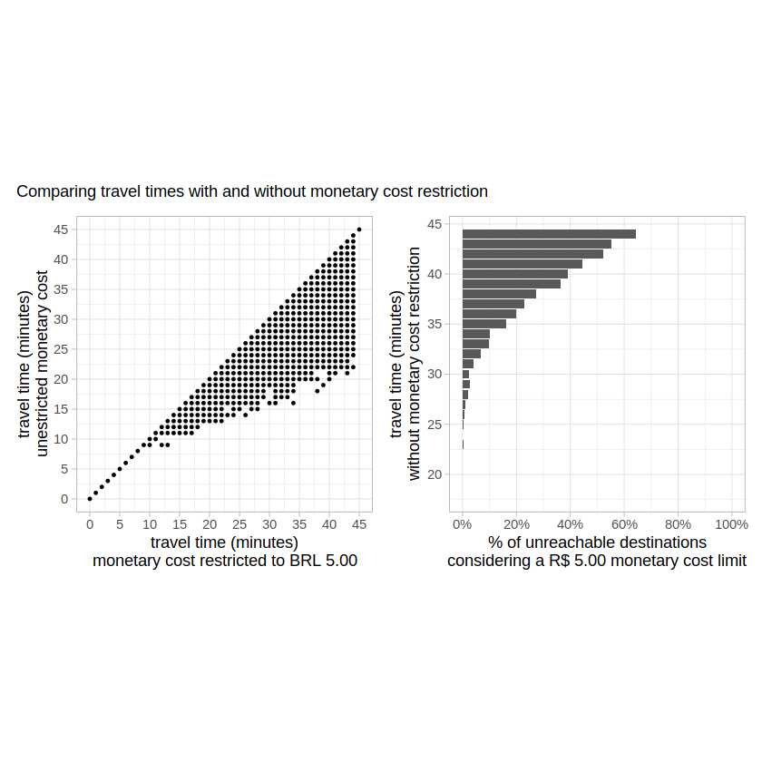
Below, we can see a sample of the travel time differences with and without monetary cost restriction. We can see that some trips are not affected at all (travel_time_unl == travel_time_500), some trips take a little longer to complete (travel_time_500 > travel_time_unl), and other trips cannot be completed at all (travel_time_500 == NA).

tail(ttm, 10)

A data.table: 10 × 4
from_id	to_id	travel_time_500	travel_time_unl
<chr>	<chr>	<int>	<int>
89a90166da7ffff	89a90129c2bffff	38	36
89a90166da7ffff	89a90129aa7ffff	33	30
89a90166da7ffff	89a90e93497ffff	32	32
89a90166da7ffff	89a90129807ffff	39	38
89a90166da7ffff	89a90129b5bffff	34	34
89a90166da7ffff	89a90129dd7ffff	37	37
89a90166da7ffff	89a90129bbbffff	33	33
89a90166da7ffff	89a90129bd7ffff	26	26
89a90166da7ffff	89a90129a47ffff	19	19
89a90166da7ffff	89a90166da7ffff	0	0

The plots below show the overall distribution of the travel time differences and unreachable destinations:

# plot of overall travel time differences between limited and unlimited cost travel time matrices 
time_difference = ttm[!is.na(travel_time_500), .(count = .N), 
                      by = .(travel_time_unl, travel_time_500)]

p1 <- ggplot(time_difference, aes(y = travel_time_unl, x = travel_time_500)) +
  geom_point(size = 0.7) +
  coord_fixed() +
  scale_x_continuous(breaks = seq(0, 45, 5)) +
  scale_y_continuous(breaks = seq(0, 45, 5)) +
  theme_light() +
  theme(legend.position = "none") +
  labs(y = "travel time (minutes)\nunestricted monetary cost",
       x = "travel time (minutes)\nmonetary cost restricted to BRL 5.00"
       )

# plot of unreachable destinations when the monetary cost limit is too low
unreachable <- ttm[, .(count = .N), by = .(travel_time_unl, is.na(travel_time_500))]
unreachable[, perc := count / sum(count, na.rm = T), by = .(travel_time_unl)]
unreachable <- unreachable[is.na == TRUE]
unreachable <- na.omit(unreachable)

p2 <- ggplot(unreachable, aes(x=travel_time_unl, y=perc)) +
  geom_col() +
  coord_flip() +
  scale_x_continuous(breaks = seq(0, 45, 5)) +
  scale_y_continuous(limits = c(0, 1), breaks = seq(0, 1, 0.2), 
                     labels = paste0(seq(0, 100, 20), "%")) +
  theme_light() +
  labs(x = "travel time (minutes)\nwithout monetary cost restriction",
       y = "% of unreachable destinations\nconsidering a R$ 5.00 monetary cost limit")

# combine both plots using patchwork
p1 + p2 + plot_annotation(subtitle = "Comparing travel times with and without monetary cost restriction")

../../_images/3f74317f0fb07dabb5281234274aa9ac0243f28bab7986b8a54148a59838ca15.png

4.2 Calculating accessibility with monetary cost#

Now, we can answer questions like “how many health care facilities one can access in 60 minutes using public transport, on a R$5.00 budget?”. We’ll do that below, and compare the results the accessibility unconstrained by monetary costs:

# calculate accessibility function
calculate_accessibility <- function(fare, fare_string) {
  access_df <- accessibility(r5r_core,
                             origins = points,
                             destinations = points,
                             departure_datetime = as.POSIXct("13-05-2019 14:00:00",
                                                             format = "%d-%m-%Y %H:%M:%S"),
                             opportunities_colname = "healthcare",
                             mode = c("WALK", "TRANSIT"),
                             cutoffs = c(60),
                             fare_structure = fare_structure,
                             max_fare = fare,
                             max_trip_duration = 45,
                             max_walk_time = 30,
                             progress = FALSE)
  access_df$max_fare <- fare_string
  return(access_df)
}
# calculate accessibility, combine results, and convert to SF
access_500 <- calculate_accessibility(fare=5, fare_string="R$ 5.00 budget")
access_unl <- calculate_accessibility(fare=Inf, fare_string="Unlimited budget")
access <- rbind(access_500, access_unl)
# bring geometry
access$geometry <- h3jsr::cell_to_polygon(access$id)
access <- st_as_sf(access)

Finally, we can plot the results and see how accessibility levels can differ quite substantially when we account for monetary costs.

# plot accessibility maps
ggplot(data = access) +
  geom_sf(aes(fill = accessibility), color=NA, size = 0.2) +
  scale_fill_distiller(palette = "Spectral") +
  facet_wrap(~max_fare) +
  labs(subtitle = "Effect of monetary cost on accessibility") +
  theme_minimal() +
  theme(legend.position = "bottom",
        axis.text = element_blank())

../../_images/2cb9d905c16bfb5de1c9906437a53697daa985f4ac02ffbf46113cc599e63992.png

If you have any suggestions or want to report an error, please visit the package GitHub page.

r5r: Accounting for monetary costs

Contents

r5r: Accounting for monetary costs#

Getting started#

Run these codes in Binder#

Working with Jupyter Notebooks#

1. Introduction#

1.1 Details#

2. Reprex: the public transport system of Porto Alegre#

3. Setting up the fare structure#

3.1 Global Properties#

max_discounted_transfers#

transfer_time_allowance#

fare_cap#

3.2 Configure fares by transport mode#

3.3 Configure fares by transfers#

3.4 Routes configuration#

4. Calculating travel time and accessibiilty accounting for monetary costs#

4.1 Travel time with monetary cost#

4.2 Calculating accessibility with monetary cost#

`max_discounted_transfers`#

`transfer_time_allowance`#

`fare_cap`#