

r5r: Case Brighton - Calculate travel time matrices in R
Contents
r5r: Case Brighton - Calculate travel time matrices in R#
Lesson objectives#
This tutorial focuses on introducing you how to compute travel time matrices by different travel modes using a relatively new R-package called r5r. Travel time data is fundamental information whenever aiming to analyze e.g. accessibility -related questions.
Library status#
r5r is still developing fast but it already has many useful functionalities related to spatial accessibility analysis. r5r has at the moment more implemented functionalities compared to r5py. Eventually, both of these libraries aim to provide a similar set of functionalities.
Run these codes in Binder#
Before you can run this Notebook, and/or do any programming, you need to launch the Binder instance. You can find buttons for activating the python environment at the top-right of this page which look like this:

Working with Jupyter Notebooks#
Jupyter Notebooks are documents that can be used and run inside the JupyterLab programming environment containing the computer code and rich text elements (such as text, figures, tables and links).
A couple of hints:
You can execute a cell by clicking a given cell that you want to run and pressing Shift + Enter (or by clicking the “Play” button on top)
You can change the cell-type between
Markdown(for writing text) andCode(for writing/executing code) from the dropdown menu above.
See further details and help for using Notebooks and JupyterLab from here.
Compute travel time matrices#
When trying to understand the accessibility of a specific location, you typically want to look at travel times between multiple locations (one-to-many). Next, we will learn how to calculate travel time matrices using r5r R-package.
When calculating travel times with r5r, you typically need a few datasets:
A road network dataset from OpenStreetMap (OSM) in Protocolbuffer Binary (
.pbf) format:This data is used for finding the fastest routes and calculating the travel times based on walking, cycling and driving. In addition, this data is used for walking/cycling legs between stops when routing with transit.
Hint: Sometimes you might need modify the OSM data beforehand, e.g., by cropping the data or adding special costs for travelling (e.g., for considering slope when cycling/walking). When doing this, you should follow the instructions on the Conveyal website. For adding customized costs for pedestrian and cycling analyses, see this repository.
A transit schedule dataset in General Transit Feed Specification (GTFS.zip) format (optional):
This data contains all the necessary information for calculating travel times based on public transport, such as stops, routes, trips and the schedules when the vehicles are passing a specific stop. You can read about the GTFS standard here.
Hint:
r5rcan also combine multiple GTFS files, as sometimes you might have different GTFS feeds representing, e.g., the bus and metro connections.
Digital Elevation Model (DEM) data (optional) in GeoTIFF format (
.tif):This data is used to calculate impedance for walking and cycling based on street slopes.
You can download this data directly from USGS / NASA or use elevatr -package
Sample datasets#
In the following tutorial, we use open source datasets for Brighton & Hove:
The point dataset for this tutorial has been obtained from WorldPop -project licensed under a Creative Commons Attribution 4.0 International License.
The street network is a cropped and filtered extract of OpenStreetMap (© OpenStreetMap contributors, ODbL license)
The GTFS transport schedule dataset for Brighton are open datasets obtained from:
Bus schedules: Brighton & Hove Bus and Coach Company licensed under Open Government License Version 3.0.
Download the datasets#
We have prepared a Zip-package with all relevant data that helps you to start working with the tools quickly. You can download and extract the data by running the following cell.
# Download the data from a S3 bucket into 'data' folder
!wget -P data/ https://a3s.fi/swift/v1/AUTH_0914d8aff9684df589041a759b549fc2/R5edu/Brighton.zip

# Extract the contents
!unzip -q data/Brighton.zip -d data/
--2022-11-29 21:45:08--  https://a3s.fi/swift/v1/AUTH_0914d8aff9684df589041a759b549fc2/R5edu/Brighton.zip
Resolving a3s.fi (a3s.fi)... 86.50.254.19, 86.50.254.18
Connecting to a3s.fi (a3s.fi)|86.50.254.19|:443... connected.
HTTP request sent, awaiting response... 200 OK
Length: 68301274 (65M) [application/zip]
Saving to: ‘data/Brighton.zip’

Brighton.zip        100%[===================>]  65,14M  36,2MB/s    in 1,8s

2022-11-29 21:45:10 (36,2 MB/s) - ‘data/Brighton.zip’ saved [68301274/68301274]
If running the cell above does not work for some reason (on your local computer), you can manually download the data. If you do this, extract the contents of the Zip file (Brighton.zip) into the <YOUR_FOLDER_CONTAINING_THIS_NOTEBOOK>/data -folder.
Installation#
r5r can be installed from CRAN. However, we will be using the latest version of the tool by installing it directly from Github as follows:
# Install the CRAN version (0.7.1)
#install.packages("r5r")

# Install the latest version of the library (0.7.9)
devtools::install_github("ipeaGIT/r5r", subdir = "r-package")
Load the origin and destination data#
Let’s start by downloading a sample point dataset into a dataframe that we can use as our origin and destination locations. For the sake of this exercise, we have prepared a grid of points covering parts of Sussex. The point data also contains the number of residents of each 100 meter cell:
# Import libraries
library(sf)
library(data.table)
library(ggplot2)
library(tmap)
library(tidygeocoder)
library(leaflet)
library(dplyr)
library(osmdata)
# Specify data directory
data_path = "data/Brighton"

# Check what files we have
list.files(data_path)
- 'Brighton_pop_points_2020.gpkg'
- 'Brighton-DEM.tif'
- 'brightonhove_1667288932.zip'
- 'brightonhove.pbf'
# Load population points
pop_fp = file.path(data_path, "Brighton_pop_points_2020.gpkg")
pop_points = read_sf(pop_fp)

# Plot the points
tm_shape(pop_points) + tm_symbols(size=0.05, col="red", border.lwd=0, alpha=0.5)

Let’s also check how the attribute table of the data looks like:
# Check the first 5 rows
head(pop_points)
Next, we will geocode the address for Brighton Railway station. For doing this, we can use tidygeocoder library and its handy .geocode() -function:
# Find coordinates of the main railway station
station = data.frame(address = "Railway station, Brighton, UK")
station = geocode(station, address, method = "osm")

# Plot
m <- leaflet(station) %>%
     addTiles() %>%
     addCircles(lng = ~long, lat = ~lat, radius=80, col="red")
m
Passing 1 address to the Nominatim single address geocoder

Query completed in: 1 seconds
# Create a sf object out of the coordinates
station = st_as_sf(station, coords = c("long", "lat"), crs = "EPSG:4326")
head(station)
| address | geometry |
|---|---|
| <chr> | <POINT [°]> |
| Railway station, Brighton, UK | POINT (-0.1407393 50.82886) |
As a last thing, we need to assign a unique id for our station object:
station["id"] = 0
head(station)
| address | geometry | id |
|---|---|---|
| <chr> | <POINT [°]> | <dbl> |
| Railway station, Brighton, UK | POINT (-0.1407393 50.82886) | 0 |
Prepare a routable network with r5r#
Next, we will prepare the routable network with
r5r. First, we will allow the r5 engine to use 6 Gb of memory. Then we import ther5rlibrary and prepare the routable network by callingsetup_r5()-function:
# Allow 6 GiB of memory
options(java.parameters = "-Xmx6G")
# After allocating the memory import the r5r
library(r5r)
# Create the routable network by indicating the path where OSM, GTFS and possible DEM data are stored
r5r_core = setup_r5(data_path = data_path)
Using cached R5 version from /home/hentenka/.conda/envs/mamba/envs/r5edu/lib/R/library/r5r/jar/r5-v6.7-all.jar


Finished building network.dat at data/Brighton/network.dat
Calculate travel time matrix#
After building the routable network, we can do the routing. For this, we need to have x and y columns for both origins and destinations:
# Parse the lat, lon coordinates (i.e. y, x)
station[c("x", "y")] = st_coordinates(station)
head(station)
| address | geometry | id | x | y |
|---|---|---|---|---|
| <chr> | <POINT [°]> | <dbl> | <dbl> | <dbl> |
| Railway station, Brighton, UK | POINT (-0.1407393 50.82886) | 0 | -0.1407393 | 50.82886 |
# Our population points already has the `x` and `y` columns
head(pop_points)
| x | y | population | id | geom |
|---|---|---|---|---|
| <dbl> | <dbl> | <dbl> | <dbl> | <POINT [°]> |
| -0.4991666 | 50.97250 | 10.112679 | 0 | POINT (-0.4991666 50.9725) |
| -0.4991666 | 50.97167 | 19.579712 | 1 | POINT (-0.4991666 50.97167) |
| -0.4991666 | 50.97083 | 12.178864 | 2 | POINT (-0.4991666 50.97083) |
| -0.4991666 | 50.96833 | 5.552000 | 3 | POINT (-0.4991666 50.96833) |
| -0.4991666 | 50.96750 | 2.551825 | 4 | POINT (-0.4991666 50.9675) |
| -0.4991666 | 50.96667 | 2.637614 | 5 | POINT (-0.4991666 50.96667) |
# Set parameters
mode = c("WALK", "TRANSIT")
max_walk_time = 30 # minutes
max_trip_duration = 120 # minutes
departure_datetime = as.POSIXct("01-12-2022 8:30:00",
                                 format = "%d-%m-%Y %H:%M:%S")

# Calculate the travel time matrix by Transit
ttm = travel_time_matrix(r5r_core = r5r_core,
                          origins = station,
                          destinations = pop_points,
                          mode = mode,
                          departure_datetime = departure_datetime,
                          max_walk_time = max_walk_time,
                          max_trip_duration = max_trip_duration)

head(ttm)
Warning message in assign_points_input(origins, "origins"):
“'origins$id' forcefully cast to character.”
Warning message in assign_points_input(destinations, "destinations"):
“'destinations$id' forcefully cast to character.”
| from_id | to_id | travel_time_p50 |
|---|---|---|
| <chr> | <chr> | <int> |
| 0 | 8549 | 112 |
| 0 | 8550 | 113 |
| 0 | 8551 | 113 |
| 0 | 8552 | 114 |
| 0 | 8553 | 112 |
| 0 | 8554 | 112 |
Now we can join the travel time information back to the population points
# Convert 'to_id' back to integer which is needed for the join
ttm[, to_id:=as.numeric(to_id)]

# Make inner join - the key in left is 'id' and in right 'to_id'
geo = inner_join(pop_points, ttm, by=c(id = "to_id"))
head(geo)
| x | y | population | id | geom | from_id | travel_time_p50 |
|---|---|---|---|---|---|---|
| <dbl> | <dbl> | <dbl> | <dbl> | <POINT [°]> | <chr> | <int> |
| -0.3366666 | 50.88750 | 4.990854 | 8549 | POINT (-0.3366666 50.8875) | 0 | 112 |
| -0.3366666 | 50.88667 | 6.199840 | 8550 | POINT (-0.3366666 50.88667) | 0 | 113 |
| -0.3366666 | 50.88583 | 10.519016 | 8551 | POINT (-0.3366666 50.88583) | 0 | 113 |
| -0.3366666 | 50.88500 | 13.427657 | 8552 | POINT (-0.3366666 50.885) | 0 | 114 |
| -0.3366666 | 50.88417 | 13.396514 | 8553 | POINT (-0.3366666 50.88417) | 0 | 112 |
| -0.3366666 | 50.88333 | 7.725784 | 8554 | POINT (-0.3366666 50.88333) | 0 | 112 |
Finally, we can visualize the travel time map and investigate how the railway station in Brighton can be accessed from different parts of the region, by public transport.
# Plot the travel times
tm_shape(geo) + tm_symbols(col="travel_time_p50", size=0.5, border.lwd=0)

Calculate travel times by bike#
In a very similar manner, we can calculate travel times by cycling. We only need to modify our TravelTimeMatrixComputer object a little bit. We specify the cycling speed by using the parameter speed_cycling and we change the transport_modes parameter to correspond to [LegMode.BICYCLE. This will initialize the object for cycling analyses:
# Define parameters
mode = "BICYCLE"
max_trip_duration = 120 # minutes
max_bike_time = 120 # minutes
departure_datetime <- as.POSIXct("01-12-2022 8:30:00",
                                 format = "%d-%m-%Y %H:%M:%S")
bike_speed = 16 # km/h

# Calculate the travel time matrix by Transit
ttm = travel_time_matrix(r5r_core = r5r_core,
                          origins = station,
                          destinations = pop_points,
                          mode = mode,
                          departure_datetime = departure_datetime,
                          max_bike_time = max_bike_time,
                          max_trip_duration = max_trip_duration,
                          bike_speed = bike_speed
                        )

head(ttm)
Warning message in assign_points_input(origins, "origins"):
“'origins$id' forcefully cast to character.”
Warning message in assign_points_input(destinations, "destinations"):
“'destinations$id' forcefully cast to character.”
| from_id | to_id | travel_time_p50 |
|---|---|---|
| <chr> | <chr> | <int> |
| 0 | 6174 | 119 |
| 0 | 6247 | 119 |
| 0 | 6316 | 119 |
| 0 | 6380 | 120 |
| 0 | 6437 | 120 |
| 0 | 6438 | 119 |
Let’s again make a table join with the population grid
# Convert 'to_id' back to integer which is needed for the join
ttm[, to_id:=as.numeric(to_id)]

# Make inner join - the key in left is 'id' and in right 'to_id'
geo = inner_join(pop_points, ttm, by=c(id = "to_id"))
head(geo)
| x | y | population | id | geom | from_id | travel_time_p50 |
|---|---|---|---|---|---|---|
| <dbl> | <dbl> | <dbl> | <dbl> | <POINT [°]> | <chr> | <int> |
| -0.3941666 | 50.80667 | 20.31480 | 6174 | POINT (-0.3941666 50.80667) | 0 | 119 |
| -0.3933333 | 50.80667 | 20.58511 | 6247 | POINT (-0.3933333 50.80667) | 0 | 119 |
| -0.3925000 | 50.80667 | 20.49868 | 6316 | POINT (-0.3925 50.80667) | 0 | 119 |
| -0.3916666 | 50.80833 | 26.29699 | 6380 | POINT (-0.3916666 50.80833) | 0 | 120 |
| -0.3908333 | 50.80917 | 25.50407 | 6437 | POINT (-0.3908333 50.80917) | 0 | 120 |
| -0.3908333 | 50.80833 | 25.89168 | 6438 | POINT (-0.3908333 50.80833) | 0 | 119 |
And plot the data
# Plot the travel times
tm_shape(geo) + tm_symbols(col="travel_time_p50", size=0.5, border.lwd=0)

Calculate catchment areas#
One quite typical accessibility analysis is to find out catchment areas for multiple locations, such as schools. In the below, we will extract all libraries in Brighton area and calculate travel times from all grid cells to the closest one. As a result, we have catchment areas for each school.
Let’s start by preparing data. In the following, we will:
Download OSM data about locations of schools in Brighton area, using
osmdata-package.We will also rename the column
osm_idtoidbecauser5rexpects to find a unique-id from columnid(similarly asr5py)Lastly, we will extract the x and y coordinates from the geometries
# Extent of the data for Brighton
# (minx, miny, maxx, maxy)
bounds = c(-0.49975, 50.73,  0.3469234, 50.98)

# Retrieve schools from OSM
schools = opq(bbox = bounds) |>
  add_osm_feature(key = "amenity", value="school") |>
  osmdata_sf()

# Keep only `osm_polygons` object from the result
schools = schools$osm_polygons

# Rename 'osm_id' to 'id'
schools = rename(schools, id=osm_id)

# Extract the lat and lon coordinates of the Polygon centroids
schools[c("lon", "lat")] = st_coordinates(st_centroid(schools))
head(schools)
Warning message in st_centroid.sf(schools):
“st_centroid assumes attributes are constant over geometries of x”
| id | name | addr.city | addr.country | addr.housename | addr.housenumber | addr.locality | addr.place | addr.postcode | addr.province | geometry | ⋯ | start_date | surface | toilets.wheelchair | website | wheelchair | wikidata | wikipedia | geometry | lon | lat | |
|---|---|---|---|---|---|---|---|---|---|---|---|---|---|---|---|---|---|---|---|---|---|---|
| <chr> | <chr> | <chr> | <chr> | <chr> | <chr> | <chr> | <chr> | <chr> | <chr> | ⋯ | <chr> | <chr> | <chr> | <chr> | <chr> | <chr> | <chr> | <POLYGON [°]> | <dbl> | <dbl> | ||
| 4564528 | 4564528 | Brighton College Sports Ground | NA | NA | NA | NA | NA | NA | NA | NA | POLYGON ((-0.0958142 50.820... | ⋯ | NA | NA | NA | NA | NA | NA | NA | POLYGON ((-0.0958142 50.820... | -0.09774609 | 50.81997 |
| 4796362 | 4796362 | Burgess Hill Girls | Burgess Hill | NA | NA | NA | NA | NA | RH15 0EG | NA | POLYGON ((-0.1259993 50.950... | ⋯ | NA | NA | NA | NA | NA | NA | NA | POLYGON ((-0.1259993 50.950... | -0.12438086 | 50.95140 |
| 22767691 | 22767691 | Herstmonceux Church of England Primary School | NA | NA | NA | NA | NA | NA | BN27 4LG | NA | POLYGON ((0.3223906 50.8892... | ⋯ | NA | NA | NA | https://www.herstmonceux.e-sussex.sch.uk/ | NA | Q66223920 | NA | POLYGON ((0.3223906 50.8892... | 0.32290302 | 50.88901 |
| 23003318 | 23003318 | East Preston Schools | NA | NA | NA | NA | NA | NA | NA | NA | POLYGON ((-0.4829187 50.813... | ⋯ | NA | NA | NA | NA | NA | NA | NA | POLYGON ((-0.4829187 50.813... | -0.48161284 | 50.81270 |
| 23261552 | 23261552 | Ratton School | Eastbourne | NA | NA | NA | NA | NA | BN21 2XR | NA | POLYGON ((0.2611432 50.7898... | ⋯ | NA | NA | NA | http://www.ratton.e-sussex.sch.uk | NA | Q7296036 | en:Ratton School | POLYGON ((0.2611432 50.7898... | 0.25971056 | 50.79073 |
| 25772335 | 25772335 | Longhill High School | Brighton | NA | NA | NA | NA | NA | BN2 7FR | NA | POLYGON ((-0.067842 50.8190... | ⋯ | NA | NA | NA | http://www.longhill.org.uk/ | NA | Q6673876 | NA | POLYGON ((-0.067842 50.8190... | -0.06654489 | 50.81820 |
# Plot the data
m <- leaflet(schools) %>%
     addTiles() %>%
     addCircles(lng = ~lon, lat = ~lat, radius=20, col="blue")
m
As a last thing, we need to convert the sf object into a regular data.frame, which we can do by dropping the geometry column:
schools = schools %>% st_drop_geometry()
class(schools)
Next, we can initialize our travel time matrix calculator using the libraries as the origins:
# Set parameters
mode = c("WALK", "TRANSIT")
max_walk_time = 30 # minutes
max_trip_duration = 120 # minutes
departure_datetime = as.POSIXct("01-12-2022 8:30:00",
                                 format = "%d-%m-%Y %H:%M:%S")

# Calculate the travel time matrix by Transit
ttm = travel_time_matrix(r5r_core = r5r_core,
                          origins = schools,
                          destinations = pop_points,
                          mode = mode,
                          departure_datetime = departure_datetime,
                          max_walk_time = max_walk_time,
                          max_trip_duration = max_trip_duration)

head(ttm)
Warning message in assign_points_input(destinations, "destinations"):
“'destinations$id' forcefully cast to character.”
| from_id | to_id | travel_time_p50 |
|---|---|---|
| <chr> | <chr> | <int> |
| 4564528 | 10559 | 119 |
| 4564528 | 10579 | 119 |
| 4564528 | 10584 | 119 |
| 4564528 | 10602 | 119 |
| 4564528 | 10603 | 119 |
| 4564528 | 10604 | 118 |
# How many rows do we have?
nrow(ttm)
As we can see, there are more than 2 million rows of data, which comes as a result of all connections between origins and destinations. Next, we want aggregate the data and keep only travel time information to the closest school:
# Find out the travel time to closest school
closest = aggregate(ttm$travel_time_p50, by=list(ttm$to_id), FUN=min, na.rm=TRUE)
# Rename columns
closest = closest %>% rename(time=x, id=Group.1)
class(closest)
head(closest)
| id | time | |
|---|---|---|
| <chr> | <int> | |
| 1 | 10 | 4 |
| 2 | 100 | 3 |
| 3 | 10000 | 21 |
| 4 | 10001 | 19 |
| 5 | 10002 | 16 |
| 6 | 10003 | 15 |
# Convert 'to_id' back to integer which is needed for the join
closest["id"] = as.integer(closest$id)
head(closest)
| id | time | |
|---|---|---|
| <int> | <int> | |
| 1 | 10 | 4 |
| 2 | 100 | 3 |
| 3 | 10000 | 21 |
| 4 | 10001 | 19 |
| 5 | 10002 | 16 |
| 6 | 10003 | 15 |
Then we can make a table join with the grid in a similar manner as previously and visualize the data:
# Make inner join - the key in left is 'id' and in right 'to_id'
geo = inner_join(pop_points, closest, by="id")
head(geo)
| x | y | population | id | geom | time |
|---|---|---|---|---|---|
| <dbl> | <dbl> | <dbl> | <dbl> | <POINT [°]> | <int> |
| -0.4991666 | 50.96667 | 2.637614 | 5 | POINT (-0.4991666 50.96667) | 11 |
| -0.4991666 | 50.96583 | 2.588078 | 6 | POINT (-0.4991666 50.96583) | 10 |
| -0.4991666 | 50.96500 | 2.529992 | 7 | POINT (-0.4991666 50.965) | 9 |
| -0.4991666 | 50.96417 | 4.308811 | 8 | POINT (-0.4991666 50.96417) | 8 |
| -0.4991666 | 50.96333 | 7.568533 | 9 | POINT (-0.4991666 50.96333) | 6 |
| -0.4991666 | 50.96250 | 5.156054 | 10 | POINT (-0.4991666 50.9625) | 4 |
# Plot the travel times which are classified into 10 classes
tm_shape(geo) + tm_symbols(col="time", size=0.05, border.lwd=0, style="pretty", n=10, palette="RdYlBu")
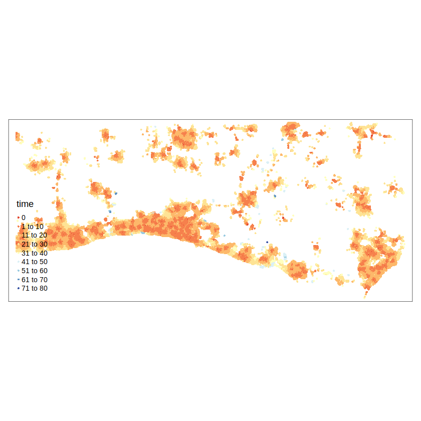
That’s it! As you can, see now we have a nice map showing the catchment areas for each school.